Simulation–Measurement Correlation in High-Frequency Planar Structures: Why They Disagree and How the Gap Is Closed
White paper · Paper 1 of a series. Why simulated and measured responses of high-frequency planar structures disagree, which factors recur, and what schools of thought exist for closing the gap.
Abstract
Simulated and measured responses of high-frequency planar structures rarely agree, and published discrepancies of 2–8% in resonant frequency are routine. This paper asks why, which factors recur, and what schools of thought exist for closing the gap.
We argue that every discrepancy has three origins: the built device differs from the simulated one, the simulation approximates the physics, and the measurement carries its own error. Drawing on three studies spanning PCB permittivity sensors to 100 GHz, additively tuned microwave sensors and silicon photonic microrings, we catalogue the recurring factors and group the remedies into five schools: higher fidelity, parameter fitting, statistical treatment, robust design and post-fabrication correction.
A case study of five setups for one simulated microstrip line shows that port type, boundary and de-embedding alone change insertion loss by a factor of 2.2 at 40 GHz. We conclude that simulation error must be bounded before a gap is attributed to manufacturing, and that agreement is better judged as a measurement falling within a predicted spread than as two curves overlapping.
1. Introduction and research question
Full-wave electromagnetic simulation is now the default way to design microwave and optical structures, yet first-pass hardware seldom matches it. Koziel and Haq survey six published resonator sensors whose measured resonances missed simulation by 1.75% to 8.43%, regardless of fabrication method or network analyser [2]. The gap is often comparable to the device's operating bandwidth, so it decides whether a design works.
The research question of this paper is:
Why do simulated and measured responses of high-frequency planar structures disagree, which factors recur across technologies, and what schools of thought exist for making them agree?
Three studies anchor the analysis:
- Lau et al. [1] quantify how copper roughness and PCB processing bias permittivity extracted from microstrip and substrate-integrated waveguide (SIW) resonators up to 100 GHz.
- Koziel and Haq [2] model fabrication and tuning errors as probability distributions and validate the predicted frequency spread against measurement.
- Mirza et al. [3] model lithographic variation in silicon microrings, including spatial correlation across a wafer, and optimise geometry to reduce its effect.
This is Paper 1 of a series. It concentrates on the simulation side of the gap: what a model assumes, omits or idealises. Manufacturing variability enters as the main reason the simulated device is not the built one.
2. A framework: three origins of discrepancy
A simulation and a measurement are two independent estimates of one device, so their difference contains the errors of both. We separate it into three origins, each needing a different remedy.
| Origin | What goes wrong | Evidence |
|---|---|---|
| Input error: the built device is not the simulated one | Dimensions, materials and surfaces differ from nominal or datasheet values | Top-side roughness off the datasheet [1]; width and thickness vary across a wafer [3]; hand-cut patch sizes spread by 0.06–0.12 mm [2] |
| Model error: the simulation approximates | Omitted physics, simplified models, finite mesh, idealised ports and boundaries | Lossless-coupler assumption overstates Q [3]; mesh size counted as uncertainty [1] |
| Measurement error: the reference is imperfect | Fixtures, calibration, drift, operator, environment | Connectors and feed lines neglected [1]; at least ±0.05 GHz calibration error; temperature and humidity named [2] |
The separation matters because the remedies conflict. Refining a model reduces model error but cannot touch input error. Tightening fabrication reduces input error but leaves a flawed model flawed. A study that improves only one term may see no improvement in the total.
3. Manufacturing variability as an input problem
A simulation is run on one nominal geometry, but a process produces a population of devices scattered around it. All three studies find the scatter is structured: it has identifiable sources, follows near-normal distributions and propagates almost linearly to the output.
3.1 Surfaces and materials
Lau et al. trace the PCB case to how copper foil is made [1]. Foil is electrodeposited on a drum, leaving one smooth side and one rough side, and the rough side is laminated against the dielectric for adhesion. The datasheet roughness values are 0.4 µm (top) and 2.8 µm (dielectric side).
- Roughness is comparable to the skin depth above 10 GHz, so the conductor surface cannot be treated as a sharp boundary.
- Roughness raises surface resistance, adding loss, and inner inductance, lowering resonant frequency. Ignored, it inflates the extracted permittivity.
- Plating, etching and surface finish alter the top face. Measured top roughness differed from the datasheet by 0.118 µm on average, varying by board maker, finish and copper coverage.
- Etched-edge and via roughness could not be measured at all.
- The true permittivity of the laminate above 10 GHz is itself unknown; datasheets rarely specify it [1].
3.2 Dimensions
Dimensional variation dominates the other two studies.
- Koziel and Haq measured 20 hand-cut copper patches per target size. Errors were normal (Kolmogorov–Smirnov p of 0.6–0.8) with standard deviations of 0.060 mm and 0.121 mm [2].
- Mirza et al. cite width and thickness standard deviations of 3.9 nm and 1.3 nm for a 248 nm lithography process. One nanometre of thickness shifts a microring resonance by about 2 nm, against channel spacings as small as 0.8 nm [3].
3.3 Spatial and batch structure
Variation is not independent from device to device. Mirza et al. report variation within a die, between dies, wafers and lots, correlated over distance and growing from wafer centre to edge [3]. Two devices placed 50 µm apart track each other closely; at 2 mm they do not. A single simulation cannot represent this, and a single measured sample cannot characterise it.
3.4 Sensitivity depends on geometry
The same process variation harms some structures far more than others. In Lau's study, assuming a single effective roughness gave a mean permittivity error of 1.15% for microstrip resonators but 0.32% for SIW cavities, and loss tangent errors of 38% and 29% [1]. The difference is where the field sits: microstrip fields touch the top face and etched edges, while SIW fields stay in the dielectric and touch only the unaltered dielectric-side copper.
4. The simulation as a source of error
Even with perfect inputs, a simulation differs from reality through what it assumes, omits and discretises. The three studies document several such model errors, and our case study shows that setup choices alone can rival manufacturing effects.
4.1 Model errors in the literature
- Idealised conductors. A smooth-conductor or single-roughness model misstates both loss and inductance [1].
- Idealised components. A lossless-coupler assumption made simulated microring Q-factors exceed the measured 500–1800; fabricated waveguides also lost about 3 dB/cm [3].
- Simplified quantities. Averaging the effective index of unequal ring and bus waveguides is an explicit approximation [3].
- Omitted structures. Connectors and feed lines were left out of the extraction model, with the error "assumed to be small" [1].
- Discretisation. Finite mesh-cell size enters the uncertainty budget [1].
- Wrong nominal inputs. Designs simulated with the datasheet permittivity of 3.48 drifted from measurement at higher frequencies [1].
4.2 Case study: five setups for one microstrip line
We simulated a short microstrip line from 1 to 40 GHz under five setups, changing one choice at a time: line impedance (50 vs 70 Ω), solution region (open vs airbox), port type (lumped vs wave) and de-embedding (full vs shortened line with ports de-embedded). Insertion loss is reported per millimetre.
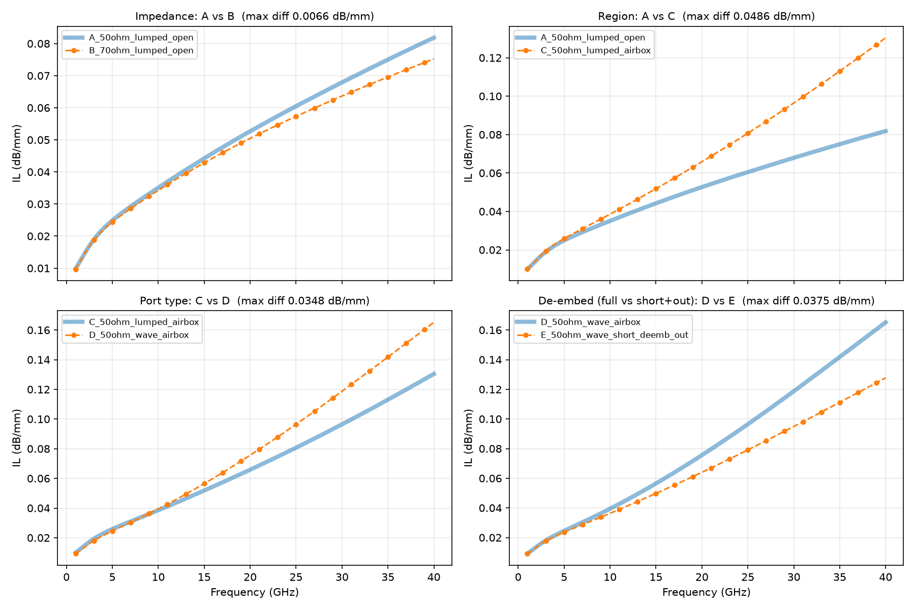
| Comparison | Setting changed | Max difference (dB/mm) |
|---|---|---|
| A vs C | Open region → airbox | 0.0486 |
| D vs E | Full line → short line, de-embedded | 0.0375 |
| C vs D | Lumped port → wave port | 0.0348 |
| A vs B | 50 Ω → 70 Ω line | 0.0066 |
At 40 GHz the five setups span roughly 0.075 to 0.165 dB/mm, a factor of about 2.2, with no change to geometry or materials. Three of the four choices are numerical, not physical, yet each moves the answer more than the 20 Ω impedance change does.
4.3 Why a short line magnifies setup error
The simulated line is short: total S21 is only 0.04–0.08 dB, implying a length near 0.5 mm. At that scale, port and launch effects are a large share of the total.
- Mismatch alone, at S11 of −30 dB, accounts for about 0.004 dB, roughly 10% of the lowest-loss case.
- The de-embedding comparison removes 0.0375 dB/mm, showing how much of the "line loss" belonged to the ports.
- From general solver practice rather than these papers: an adaptive-mesh convergence target of 0.01 in S-parameter magnitude corresponds to about 0.09 dB in |S21| near unity, larger than the loss being resolved. The convergence setting should be checked before any of these differences are taken as physical.
The curve shapes also differ. Cases A and B flatten with frequency, as conductor loss would, while C, D and E keep climbing, suggesting the airbox setups capture an additional loss mechanism. Which is closer to reality can only be settled against measurement.
5. Schools of thought on closing the gap
The literature closes the gap in five distinct ways, and they differ in what they believe the gap is. The first two treat it as a modelling defect; the last three accept it as a property of manufacturing.
| School | Underlying belief | Method | Main weakness |
|---|---|---|---|
| Higher fidelity | The model lacks detail | Measure the built part and simulate it as built: actual dimensions, metal thickness, per-face roughness [1] | Fails when a needed input cannot be measured, such as edge roughness [1] |
| Parameter fitting | Adjust inputs until curves agree | Sweep permittivity or roughness and interpolate to the measured response [1] | Fitted values absorb unrelated errors and transfer only to similar geometries [1] |
| Statistical treatment | A single match is the wrong target | Predict a distribution of outcomes; test whether measurement falls inside it [2], [3] | Needs variation data and many samples |
| Robust design | Make the gap matter less | Choose structures or dimensions with low sensitivity [1], [3] | Costs coupling, bandwidth or area [3] |
| Post-fabrication correction | Fix the hardware, not the model | Tune or trim each device after measuring it [2] | Labour or power per device; doesn't scale [2], [3] |
A sixth approach, improving the measurement itself, is common practice but only touched on in these papers. Lau et al. average ten sweeps, repeat on another day with fresh calibration, and note that probes would avoid connector effects [1].
5.1 The case against fitting
Lau's paper is in effect a critique of fitting. A permittivity extracted from a microstrip resonator with the wrong roughness assumption is a "design permittivity": it bundles conductor and geometry effects into the material value [1]. The fit is exact for that structure and wrong for the next.
Adding detail does not rescue it. Measured roughness values only "slightly" improved microstrip results, because edge roughness remained unknown [1]. When an input is unobtainable, fidelity has a ceiling.
5.2 Design before versus correction after
Robust design and post-fabrication correction answer the same problem at different times. Lau switches structure so the unknown surfaces drop out; Mirza keeps the structure and searches its dimensions, and a wider microring cut average measured resonance shift from 7.1 nm to 1.8–2.1 nm [3]. Koziel accepts the error and tunes each sensor, reaching 0.01 GHz after 10–20 placement attempts [2].
6. Statistical treatment: the variance budget
Koziel and Haq [2] and Mirza et al. [3] share one method, which turns "why doesn't it match?" into a testable prediction. It has four steps.
- Describe each input as a distribution. Estimate mean and standard deviation from fabricated samples or the vendor, and check normality (Koziel uses Kolmogorov–Smirnov tests and Q–Q plots).
- Get each sensitivity from the solver. Perturb one parameter and record the output change, e.g. Δf/ΔS ≈ 1.02 GHz/mm for patch size [2], or ∂λ/∂w by central difference [3].
- Propagate. Output spread from one input is its sensitivity times its standard deviation.
- Combine. For independent sources:
Koziel combines in quadrature, as above. Mirza sums the terms linearly, a worst-case bound that is more conservative.
6.1 How well it predicts
Koziel's prediction held within a factor of about 1.4:
| Target patch | Predicted mean shift (GHz) | Predicted σ (GHz) | Measured mean shift (GHz) | Measured σ (GHz) |
|---|---|---|---|---|
| 1.5 mm | 0.08 | 0.096 | −0.08 | 0.132 |
| 2.0 mm | 0.00 | 0.184 | 0.05 | 0.163 |
The spreads agree reasonably; the means do not always agree in sign. That residual is a systematic offset the budget does not capture, consistent with the ±0.05 GHz calibration error the authors report [2].
6.2 What changes in the question
Under this treatment, correlation no longer means overlapping curves. It means the measured value lies within the predicted interval, and the interval is narrow enough to be useful. A simulation can then be "right" while missing a given sample, and "wrong" while matching one by chance.
The method has limits. It is first-order, so it assumes the response is near-linear in each input, which Mirza confirms for microrings over ±10 nm [3]. It assumes independence, which spatial correlation violates [3]. And it propagates input error only: model error and measurement error need their own terms.
7. Application to microstrip transmission lines
Microstrip is the hardest case for correlation: Lau et al. found it the most sensitive structure to process non-idealities [1]. Applying the three design-side schools to a broadband line gives a concrete correlation programme. None of the papers works this example directly; it is our application of their logic.
| Avoid the unknowns (after [1]) | Low-sensitivity dimensions (after [3]) | Correct after fabrication (after [2]) | |
|---|---|---|---|
| When | Before fabrication | Before fabrication | After fabrication |
| Targets | Edge and top-face roughness, surface finish | Trace width, dielectric thickness, copper thickness | The residual gap on the built line |
| Actions | Wider trace, so less current on unknown edges; keep finish and solder mask off the line; smoother foil; extract roughness and true permittivity once from test structures | Perturb each parameter in the solver; weight each sensitivity by the fabricator's σ; choose the 50 Ω width–thickness pair with the smallest total | Coupons on the same panel; fit effective roughness and permittivity; measure several to get the spread; two line lengths to cancel connectors |
| Limit | A waveguide cavity, Lau's full answer, has a cutoff and cannot carry a broadband line | Thicker substrates radiate and support unwanted modes sooner at 40 GHz | Loss can be characterised, not reduced |
| Role in the argument | Explains the residual no budget can close | Provides the variance budget | Provides the validation |
Two cautions follow from Lau. Effective roughness for microstrip depends on linewidth and frequency, so a value fitted on one coupon should be reused only for similar lines [1]. And loss tangent extraction from planar structures was judged unreliable under these uncertainties, so a correlation study built on insertion loss carries the largest residual of any quantity [1].
8. Discussion and limitations
The central finding is an ordering problem. Most correlation studies attribute the residual gap to manufacturing, but that attribution is only valid once model error is bounded. Section 4 shows model error from setup choices alone can exceed plausible manufacturing effects for a short line.
The schools are complementary rather than rival. A defensible correlation study would bound model error first (convergence and setup sensitivity), build a variance budget from fabricator tolerances, design for low sensitivity where the application allows, and validate against several measured samples rather than one.
Limitations of this paper:
- Three sources. The evidence base is three studies in different technologies. Patterns common to all three are well supported; quantitative transfer between them is not.
- Case study is simulation only. The five setups in Section 4 have no measured counterpart yet, so they show which setup choices matter, not which is correct.
- Inferred geometry. The case-study line length (about 0.5 mm) is inferred from the ratio of total S21 to loss per millimetre.
- Measurement error under-treated. It is named in the framework but not analysed in depth; Paper 1 concentrates on the simulation side.
9. Conclusion
Simulation and measurement disagree because the built device is not the simulated one, the simulation approximates the physics, and the measurement is imperfect. Manufacturing variability drives the first: copper roughness that differs by face and is altered by processing, dimensions that scatter normally around nominal, and variation that is spatially correlated.
Five schools address the gap. Higher fidelity and fitting try to make one curve match another, and both fail when a needed input cannot be measured. Statistical treatment, robust design and post-fabrication correction accept variation as real and respectively predict it, reduce sensitivity to it, or remove it per device.
For microstrip insertion loss, we recommend bounding solver-setup error before attributing any gap to manufacturing, and judging correlation by whether measurements fall inside a predicted spread. Later papers in this series will address the measurement side.
References
- I. Lau, A. Hajian, F. Michler, G. Gold, F. Lurz, U. Schmid, K. Helmreich, R. Weigel and A. Koelpin, "Influence of the PCB manufacturing process on the measurement error of planar relative permittivity sensors up to 100 GHz," IEEE Trans. Microw. Theory Techn., vol. 67, no. 7, pp. 2793–2804, Jul. 2019, doi:10.1109/TMTT.2019.2910114.
- S. Koziel and T. Haq, "Uncertainty quantification of additive manufacturing post-fabrication tuning of resonator-based microwave sensors," Measurement, vol. 216, 112952, 2023, doi:10.1016/j.measurement.2023.112952.
- A. Mirza, F. Sunny, P. Walsh, K. Hassan, S. Pasricha and M. Nikdast, "Silicon photonic microring resonators: A comprehensive design-space exploration and optimization under fabrication-process variations," IEEE Trans. Comput.-Aided Design Integr. Circuits Syst., vol. 41, no. 10, pp. 3359–3372, Oct. 2022, doi:10.1109/TCAD.2021.3132555.